One Click to Polygon: SAM2-Powered Satellite Labeling

Labeling one solar panel in satellite imagery takes 30-60 seconds of careful polygon drawing. Labeling ten thousand takes a team and weeks. TerraLabel combines Meta's SAM2 segmentation model with interactive web mapping to turn that into a single click per object—100-500ms on GPU, accurate enough to replace manual tracing for most use cases.

Manual vs. Automated vs. Human-in-the-Loop

Training ML models for remote sensing demands labeled data at scale. Solar panel detection for energy audits, building footprint extraction for urban planning, agricultural parcel mapping—all require precise polygon boundaries around each object.

Fully manual digitization is accurate but costs $0.10-0.50 per polygon at production rates. Fully automated segmentation is fast but produces error rates of 15-30% that require costly review. TerraLabel takes a third approach: AI-assisted human-in-the-loop labeling. SAM2 handles boundary tracing; humans handle judgment calls. The result is 5-10x faster throughput with comparable accuracy to manual work.

Three-Tier Architecture: Svelte + FastAPI + PostGIS

TerraLabel connects a Svelte frontend with deck.gl mapping, a FastAPI backend running SAM2 inference on the 224MB Hiera Large model, and PostgreSQL with PostGIS for spatial data storage with GIST-indexed queries.

Tech Stack

• Frontend — Svelte 5, SvelteKit, deck.gl with editable-layers, Turf.js
• Backend — FastAPI, SAM2 (Hiera Large), PostgreSQL with PostGIS
• Tile Server — Martin for vector tiles, Tippecanoe for MBTiles generation
• Infrastructure — Docker Compose, NVIDIA Container Toolkit for GPU inference

The architecture decouples concerns deliberately. The frontend handles all map interaction and polygon editing—it doesn't need to know anything about machine learning. The backend exposes a simple REST endpoint: send an image and coordinates, receive a polygon. The database stores both the raw imagery and the labeled features with full spatial indexing.

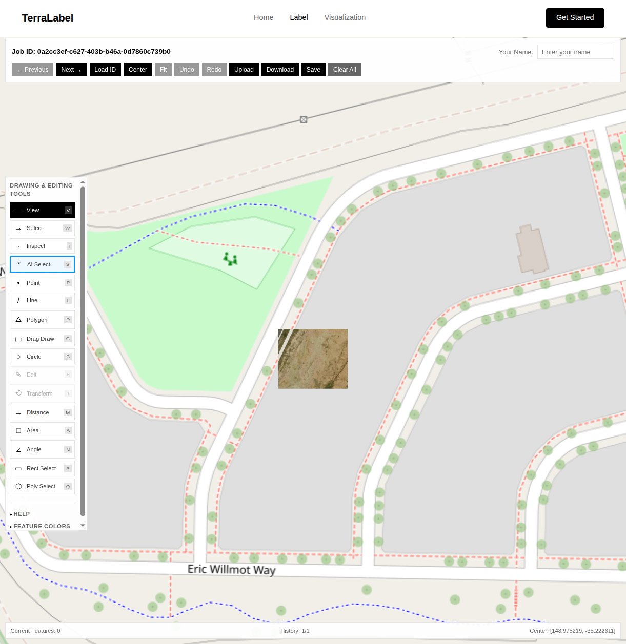
Frontend: deck.gl Editable Layers with 5 Drawing Modes

The labeling interface is built on deck.gl's editable layers, providing GIS-quality drawing tools in the browser. Users switch between AI-assisted selection and five manual drawing modes depending on the task.

In "AI Select" mode, clicking anywhere on the image sends coordinates to the backend and receives a polygon that renders immediately on the map. The full round-trip—click to rendered polygon—takes 100-500ms on GPU, 2-5 seconds on CPU.

import { EditableGeoJsonLayer } from '@deck.gl-community/editable-layers';

const editableLayer = new EditableGeoJsonLayer({
    id: 'editable-layer',
    data: featureCollection,
    mode: selectedMode, // DrawPolygonMode, ModifyMode, etc.
    selectedFeatureIndexes,

    onEdit: ({ updatedData, editType, featureIndexes }) => {
        if (editType === 'addFeature') {
            // New polygon drawn
            features = [...features, updatedData.features.at(-1)];
            pushToHistory();
        } else if (editType === 'finishMovePosition') {
            // Vertex moved
            features = updatedData.features;
            pushToHistory();
        }
    },

    getFillColor: [66, 135, 245, 100],
    getLineColor: [66, 135, 245, 255],
    getLineWidth: 2
});

The undo/redo system maintains a 50-step history by storing complete feature collection snapshots. While memory-intensive for complex annotations, this approach ensures reliable state restoration regardless of edit complexity.

Backend: SAM2 Hiera Large on FastAPI

The segmentation backend wraps Meta's 224MB SAM2 Hiera Large model in a FastAPI service. The Hierarchical Vision Transformer backbone provides multi-scale features critical for segmenting objects from small rooftop solar panels to large agricultural fields.

from sam2.sam2_image_predictor import SAM2ImagePredictor
import numpy as np
import cv2

# Load the model
predictor = SAM2ImagePredictor.from_pretrained(
    "facebook/sam2-hiera-large"
)

# Set the image (expensive operation, do once)
predictor.set_image(image_rgb)

# Predict mask from point prompt
masks, scores, logits = predictor.predict(
    point_coords=np.array([[pixel_x, pixel_y]]),
    point_labels=np.array([1]),  # 1 = foreground
    multimask_output=True
)

# Take highest-confidence mask
best_mask = masks[np.argmax(scores)]

# Extract polygon from binary mask
contours, _ = cv2.findContours(
    best_mask.astype(np.uint8),
    cv2.RETR_EXTERNAL,
    cv2.CHAIN_APPROX_SIMPLE
)

The key insight is that SAM2's image encoding is expensive (the 224MB Hiera Large model needs to process the entire image), but subsequent prompts are cheap. In an interactive workflow, we encode once when loading a job, then run lightweight prompt inference for each click.

WGS84 to Pixel Coordinate Transformation

User clicks arrive in geographic coordinates (WGS84/EPSG:4326), but SAM2 operates in pixel space. The linear interpolation is straightforward but must be applied consistently in both directions—geographic-to-pixel for click handling, pixel-to-geographic for polygon output.

def pixel_to_geographic(pixel_x, pixel_y, bounds, image_size):
    """
    Convert pixel coordinates to geographic (WGS84).

    bounds: [min_lon, min_lat, max_lon, max_lat]
    image_size: (width, height)
    """
    min_lon, min_lat, max_lon, max_lat = bounds
    width, height = image_size

    # Linear interpolation
    lng = (pixel_x / width) * (max_lon - min_lon) + min_lon
    lat = max_lat - (pixel_y / height) * (max_lat - min_lat)

    return [lng, lat]

def geographic_to_pixel(lng, lat, bounds, image_size):
    """Reverse transformation for click handling."""
    min_lon, min_lat, max_lon, max_lat = bounds
    width, height = image_size

    pixel_x = (lng - min_lon) / (max_lon - min_lon) * width
    pixel_y = (max_lat - lat) / (max_lat - min_lat) * height

    return [pixel_x, pixel_y]

API Design

The inference endpoint accepts a base64-encoded image, the geographic bounds of that image, and the click coordinates. It returns a GeoJSON polygon ready for rendering.

@app.post("/generate-label")
async def generate_label(request: LabelRequest):
    """
    Generate polygon from point click using SAM2.

    Input: base64 image, click coordinates, image bounds
    Output: GeoJSON polygon with confidence score
    """
    # Decode image
    image = decode_base64_image(request.image)

    # Transform click to pixel space
    pixel_coords = geographic_to_pixel(
        request.lng, request.lat,
        request.bounds, image.shape[:2]
    )

    # Run SAM2 inference
    mask = predict_mask(image, pixel_coords)

    # Extract and simplify polygon
    polygon = mask_to_polygon(mask, epsilon=2.0)

    # Transform back to geographic coordinates
    geojson = polygon_to_geojson(polygon, request.bounds, image.shape)

    return {"polygon": geojson, "confidence": float(scores.max())}

Polygon simplification (using Douglas-Peucker with epsilon=2.0 pixels) reduces the vertex count while preserving shape fidelity. This is important because SAM2 masks can produce jagged boundaries at pixel resolution—not useful for downstream applications.

Visualization: ~50KB Tiles vs 160MB+ Full GeoJSON

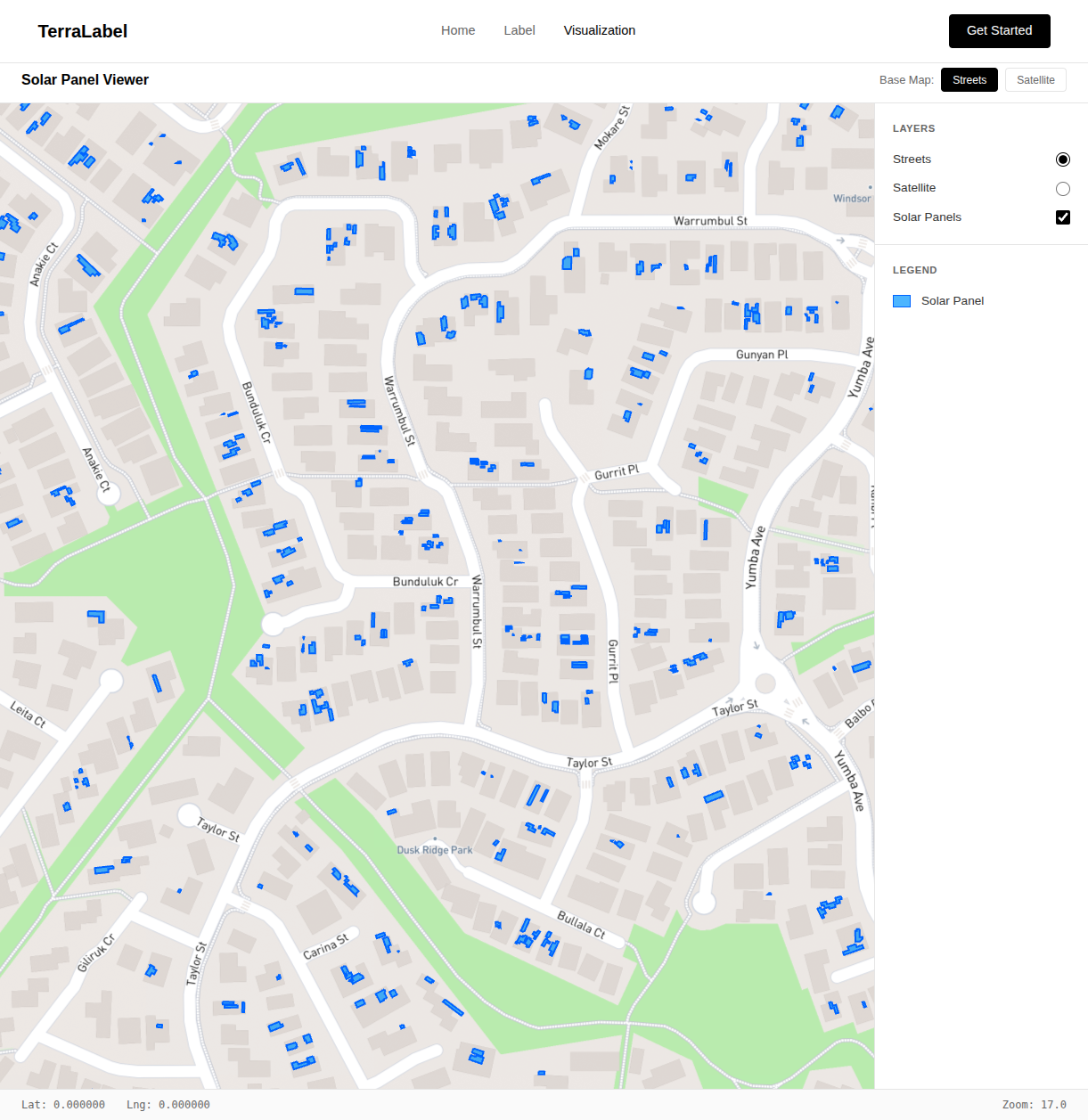
The visualization tool displays all labeled features across the entire study area. For Canberra's solar panel dataset, this means thousands of polygons that need to render smoothly at any zoom level.

Loading all features as GeoJSON would be impractical—even a moderately sized dataset becomes unwieldy in the browser. Instead, we use Martin to serve vector tiles directly from PostGIS. The database handles spatial queries, Martin generates tiles on demand, and deck.gl's MVTLayer renders them efficiently.

Database Schema

PostgreSQL with PostGIS handles both the raw imagery and labeled features. The schema stores binary satellite image tiles alongside their geographic bounds, allowing the backend to retrieve the correct imagery for any job.

Labels are stored as JSONB containing GeoJSON feature collections. This flexible schema accommodates varying numbers of features per job without requiring schema changes. PostGIS GIST indexes enable fast spatial queries for the visualization layer.

GPU vs CPU: 100ms vs 5s Inference Latency

GPU inference (NVIDIA with CUDA) delivers 100-500ms latency—imperceptible in an interactive workflow. CPU inference takes 2-5 seconds—acceptable for batch processing but disruptive for live annotation where sub-second feedback maintains labeling rhythm.

For production deployment, we use Docker Compose with NVIDIA Container Toolkit for GPU access. The frontend deploys as a static SvelteKit build, the FastAPI backend runs behind Gunicorn with Uvicorn workers, and Martin serves vector tiles.

Thousands of Solar Panels Labeled in Canberra

TerraLabel has been used to label thousands of solar panels across Canberra using high-resolution ACT government aerial imagery. The AI-assisted workflow delivered 5-10x faster throughput than manual digitization while maintaining comparable polygon accuracy.

• SAM2 generalizes well — Despite being trained on natural images, it handles satellite imagery with minimal domain shift. Solar panels, buildings, and agricultural fields all segment reliably.
• Interactive latency matters — Sub-second response times maintain flow state. Anything over 2 seconds breaks the rhythm of labeling.
• Simplification is essential — Raw SAM2 masks have pixel-level jaggedness that's useless for real applications. Douglas-Peucker smoothing is non-negotiable.
• Vector tiles scale — Moving from full GeoJSON loads to on-demand vector tiles transformed the visualization from unusable to smooth.
• Human-in-the-loop wins — Neither fully manual nor fully automatic approaches work well. AI handles the tedium; humans handle the ambiguity.

Planned: Multi-Point Prompts and Active Learning

The current system handles single-click segmentation. Future iterations will add:

• Multi-point prompts — Positive and negative clicks to refine ambiguous segmentations
• Box prompts — Bounding box selection for complex scenes with multiple candidates
• Fine-tuning — Domain adaptation using the labeled data to improve future predictions
• Active learning — Prioritizing unlabeled samples where the model is most uncertain

TerraLabel demonstrates that foundation models like SAM2 can dramatically accelerate geospatial workflows when properly integrated with domain-specific tooling. The combination of AI assistance and human judgment produces better results than either approach alone.